
Capacitor Fringing Effects and Electrostatic Simulation
01
Project Background
Finite electrode size, changing gaps and nearby grounded structures can limit a simple parallel-plate estimate. Treating a contour plot as the design conclusion can overlook outer-boundary distance, dielectric properties and local mesh effects at sharp corners.
The model uses two-dimensional electrodes and an air domain to examine why simplified estimates differ from numerical results. The scope covers electrostatic boundary-value modeling and review; manufacturing, breakdown tests and high-frequency electromagnetic compatibility require separate assessment.
02
Technical Approach and Boundary Definition
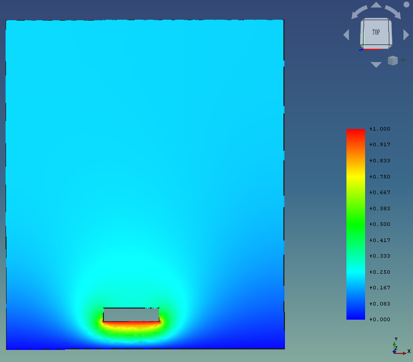
Define electrodes, dielectrics and the outer computational domain, then assign materials and equations explicitly. Register the reference potential, electrode excitation and outer-boundary conditions separately. An unassigned boundary is not automatically ground; verify how the solver treats it.
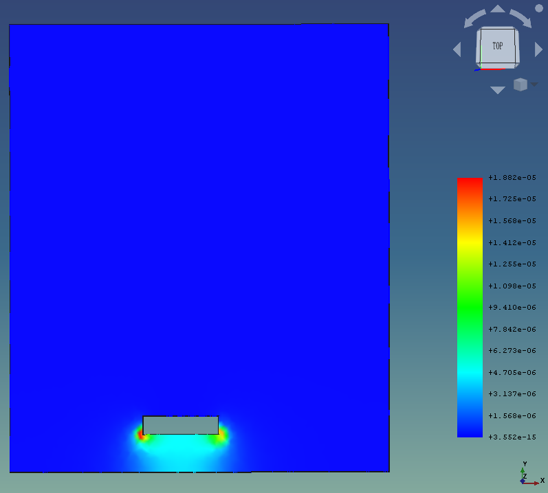
The source includes normalized settings. A real project must supply justified geometric scales, dielectric properties and units. Distinguish the solved potential from derived fields and document interpolation or averaging, so smoother visualization is not mistaken for greater local accuracy.
03
Implementation and Result Review
Generate a baseline mesh, confirm electrode selections and solve while retaining convergence records. Refine near electrodes and edges, comparing multiple meshes under unchanged geometry and boundaries to isolate discretization effects.
Then enlarge the outer domain to assess artificial-boundary effects. Capacitance evaluation requires an explicit two-dimensional unit or equivalent-length convention and a checked energy- or charge-based calculation. Alternatives must share normalization and output definitions.
04
Deliverables and Acceptance
Deliver geometry, meshes, materials and boundary registers with solver settings, field plots and comparison records. Each plot retains a legend, field name and run identifier. Derived-field reports explain the algorithm and the spatial scale on which interpretation is supported.
Acceptance checks reproduction from the delivered project and compares trends with a simple analytical approximation or trusted benchmark. For corner peaks, review fillets, mesh changes and sample locations rather than only maxima, avoiding treatment of numerical singularities as directly usable engineering loads.
05
Applicability and Extensions
The example uses normalized parameters and a two-dimensional electrostatic assumption. Three-dimensional connectors, frequency-dependent dielectrics and time-varying circuits require appropriate models and solver settings.
Dielectric loss, Joule heating or thermal deformation require additional loss models, temperature-dependent material relationships and coupling interfaces, together with corresponding tests and error checks.
06
Implementation Outcomes
The workflow makes geometry-to-boundary-to-result relationships reviewable, helping identify incorrect grounding, missing dielectric assignments and overly close outer boundaries. It supports consistent comparisons; design benefits still require validation for the target device and conditions.
Establish an efficiency baseline through boundary setup time, repeatability and rework caused by unit or face-selection errors.